
The instinct is to narrow the range. A team has too many splits on the table, and the first move is to tighten the window on each factor. It feels productive. It is not.
A full factorial with the same factors and the same number of levels costs the same number of runs however narrow the range. Narrowing changes the resolution you buy per run — it does not change the count. To reduce the number of DOE splits, you have to change the design itself.
What actually cuts the count
Three things lower the number of runs:
- Drop factors. Removing a factor divides the count by the number of levels that factor carried.
- Cut levels per factor. Going from five levels to three on one factor cuts that factor's contribution by 40%.
- Switch to a screening or fractional design instead of a full factorial.
So the real question behind "reduce the number of splits" is which factors to carry, and with how many levels. That is a screening problem: rank factors by how much they move the responses, then carry only the survivors into the expensive design.
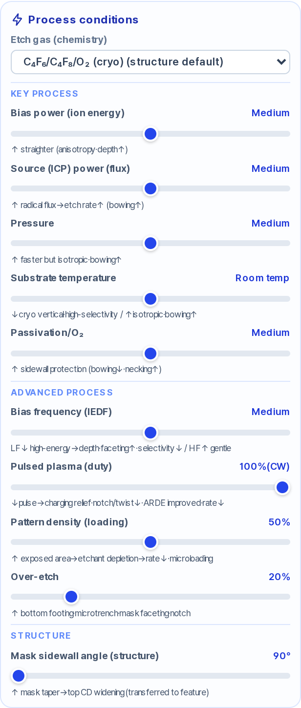
Screening costs something too — unless you can take part of it off the wafer.
What a model-based screening pass gives you
A model-based sweep can stand in for part of that first pass, because it costs no wafers. But what it shows has to be read exactly.
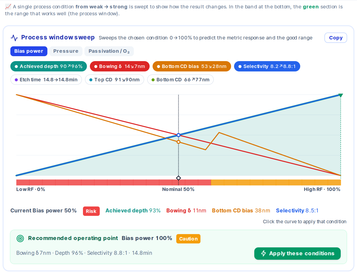
A two-factor map is a two-factor experiment. It varies two of the ten conditions the screen exposes and holds the other eight at one setting for the whole grid. A 15 × 15 grid is 225 model evaluations. Whatever it shows is conditional on where those eight sit. A one-factor sweep cannot see interactions at all; a two-factor map sees the interaction between its two factors and nothing about the rest.
There is a second limit worth stating plainly: the sweep and the map offer only three of those ten conditions as axes — bias power, pressure and passivation. So this pass cannot rank all ten factors for you. It informs the part of the screening question that falls inside those three, and leaves the rest to the physical design.
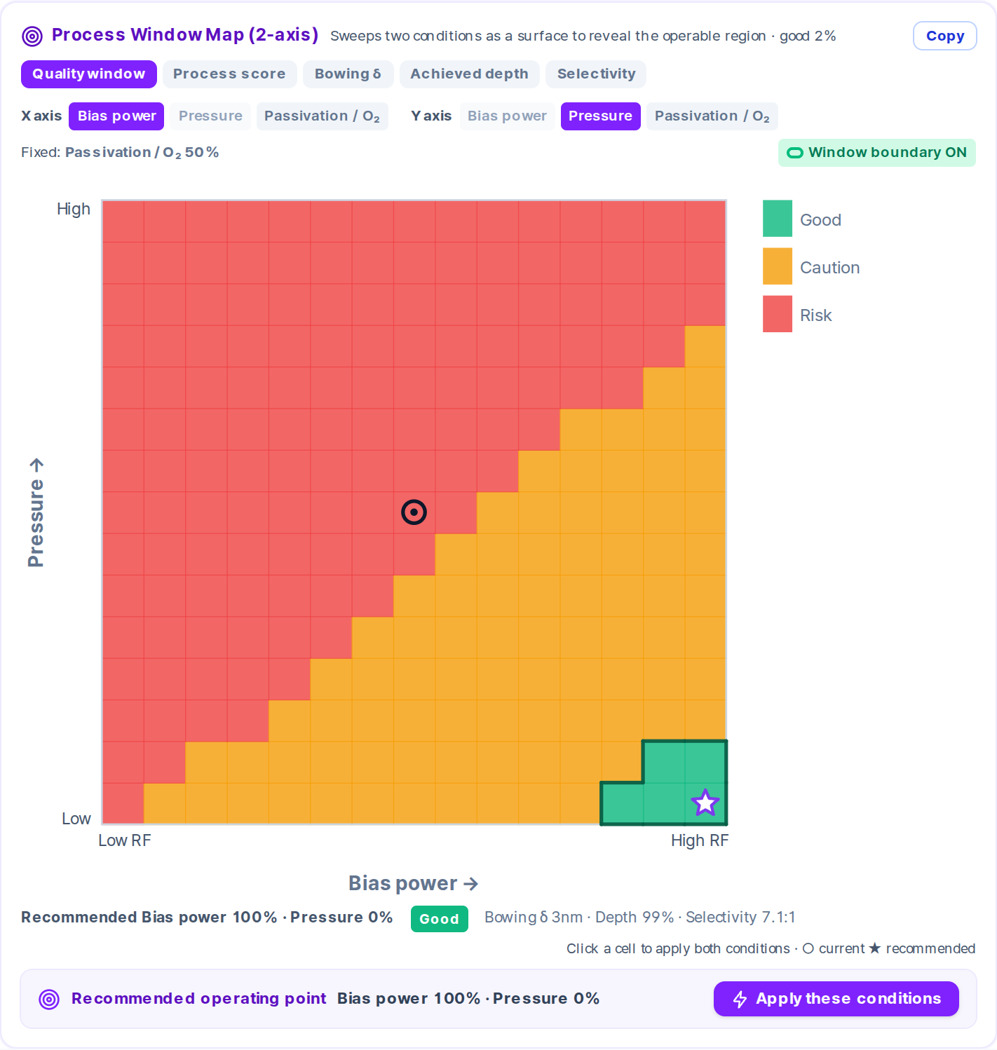
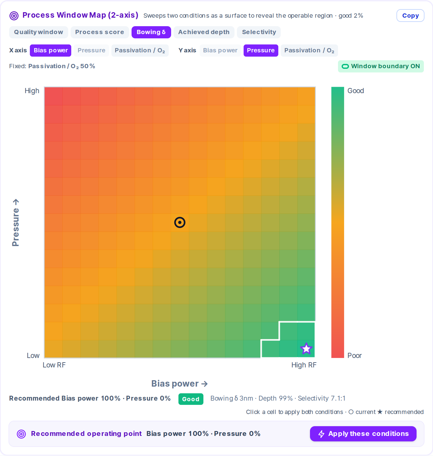
Colour means different things in different modes. One mode shows the model's good/warn/risk classification. The other four — process score, bowing delta, achieved depth, selectivity — colour each cell relative to the highest and lowest value present in that same grid. Green there means "best value in this grid", not "good": a cell the model classifies as risk can still be green. When a metric is effectively flat across the grid, every cell is drawn amber instead.
The classification tests six conditions: mask breakthrough, selectivity below 3, bowing above 22% of the half-opening, bowing above 10%, achieved depth below 90% of target, and notching. Values such as within-wafer non-uniformity or sidewall roughness are computed, but none of them is itself one of the six tests.
The recommended point is a weighted score. Achieved depth, bowing, bottom CD bias, selectivity and etch time each carry a fixed weight, with penalties for risk and caution. The weights are a choice. Different weights move the recommendation.
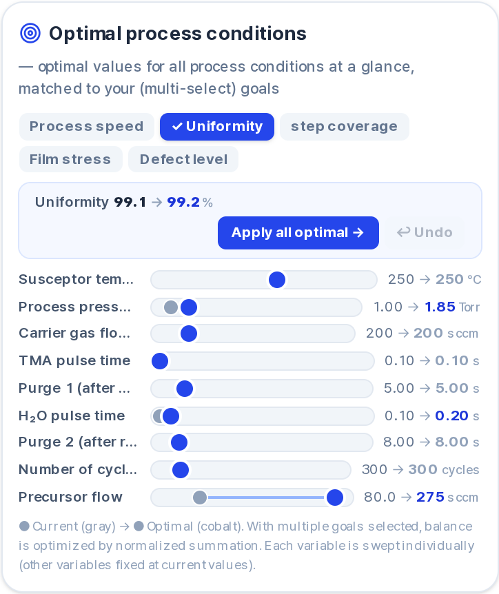
The per-variable optimiser assembles independent one-dimensional picks. For each variable in its list it walks 23 values across that variable's range while holding every other variable at its current value. Each winning value is then rounded to that variable's step, and the rounded value is not scored again. So the combined set is a candidate assembled from separate one-dimensional searches — not a joint optimum, and not guaranteed to beat where you started.
None of these grids contain wafer measurements. They are model output. A model-based pass is a screening step, not a substitute for splits: it can narrow what you carry into the physical design and show you where a model already objects. Wafers still decide. And the cheapest split remains the one you do not have to buy twice — which is what happens when the conditions behind the first run were never written down.
FAQ
Does narrowing the factor range reduce the number of runs? No. A full factorial with the same factors and levels costs the same runs regardless of range. The count falls when you drop factors, cut levels, or move to a fractional design.
Can a model-based map replace a physical DOE? No. Every value in these grids is model output. A model-based sweep can rank candidates and flag modelled risk. Confirmation still needs wafers.
What does green mean on the two-factor map? It depends on the mode. In quality-window mode it means the model classifies that cell as good. In the other four modes it means the cell holds the best value relative to the values present in that grid — a rank, not a verdict.
Why record the conditions behind every split? A split whose conditions were not recorded cannot be reused. The same question gets bought twice.
This is how we approach screening at Semi Process Lab.